Logistic Regression as a Neural Network

Notation

• 
  A single training example. Where ( is a x-dimensional feature vector), .

• or
  A training set which contains m training examples.

• 
  A test example set.

• 
  Input training example matrix which has rows and columns. .

  WARNING

  It is not a good idea to put training examples as row vectors in the matrix . It will cause much more efforts when computing.

• 
  Output matrix which has row and columns. .

Binary Classification

Logistic regression is an algorithm for binary classification (Used for the supervised learning problem which the output labels are all either 0 or 1).

Scenario example
Take a picture as an input, and want to get a label for output to infer whether the picture is a cat. Define the output label is 1 as the picture is the case of a cat picture, and the output label is 0 as the picture is the case of not a cat picture.

To Be Specific

Say, the picture is 64 × 64 pixels. And it can be divided as 3 matrices representing the red, green and blue channel.

Define the feature vector as the every elements unroll by the color matrices. So, the dimension of the feature vector is 12288. Marked as:

Goal: Classifier can predict whether the label is 1 or 0.

Logistic Regression

Example
Given a feature vector and wanting to know the probability of output label (i.e. ).

Parameters

* stand for weight, which could tell the algorithm where to focus on. stand for bias, which could make sure that the neuron will be activate meaningfully (i.e. How high the weighted sum needs to be before the neuron starts getting meaningfully active.).

Output
(Linear Regression. Will not be worked, is not between 0 and 1.)

(Sigmoid Function, i.e. )

About Sigmoid Function

The graph of sigmoid function

[Sigmoid Function]

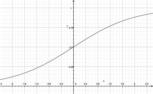
Features

Logistic Regression Cost Function

Using a cost function to train the parameters and of the logistic regression model.

Loss (Error) Function

A function used to measure how well the algorithm is doing. (For single training example)

• Square Error
  

  
  Not usually use. The optimization problem always becomes non-convex. Therefore, there will be more than one multiple local optima. It can not using for gradient descent to find the global optimum.

• Cross-Entropy Loss Function
  

  
  The lower value of loss function is, the better prediction of algorithm is.

  [Analyse]

  • If , .
    When is small, should be large, and should be large as well but no more than .
  • If , .
    When is small, should be large, and should be small but no less than .

Cost Function

A function used to measure how well the algorithm is doing. (For the whole training set)

Still, the lower value of cost function is, the better prediction of algorithm is.

Gradient Descent

A algorithm to train (learn) the parameters and on the training set. Take all the and as the parameters, the gradient descent algorithm will find out the global optimum which is the point can having the smallest value of cost function. In another word, gradient descent tells what nudges to all of the weights and biases cause the fastest change to the value of the cost function. (i.e. Which changes to weights matter the most.)

[Analyse]
Only analyse the value and parameter . Assume that the funtion is a convex function. Repeat this algorithm until the algorithm converges.

* is the learning rate. It controls how big a strep the algorithm take on each iteration.
*When writing code, will be defined as dw.

And for the real cost function, the gradient descent will be like:

*When writing code, will be defined as dw, and will be defined as db.
*Also, a coding convention dvar represent the derivative of a final output variable with respect to various intermediate quantities

Logistic Regression Gradient Descent

[Analyse]
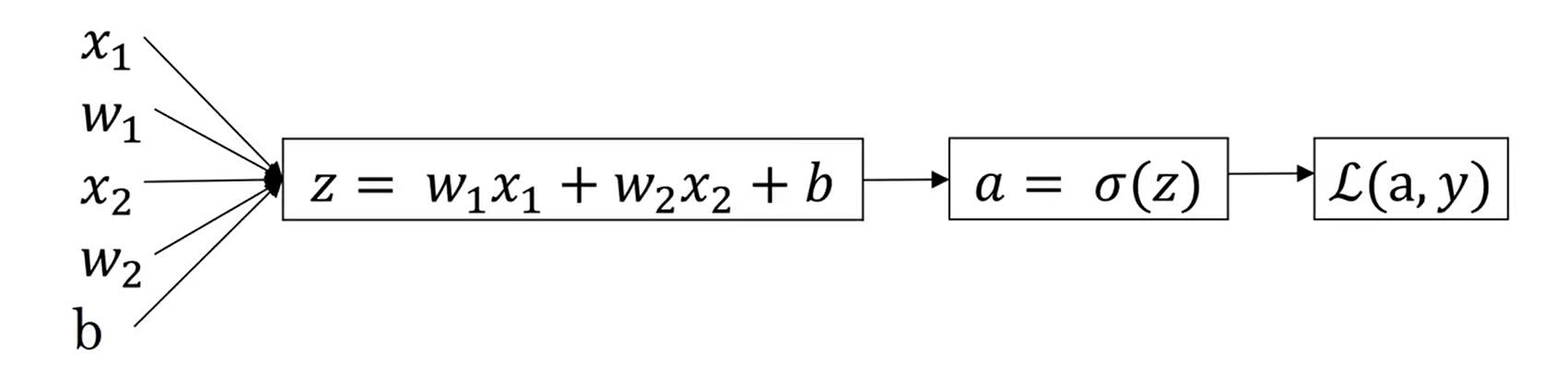
For a training example which has two features.

features: and
parameters: , and

da:

dz:

dw1:

dw2:

db:

*In this repeat loop, means dw1, and means dw2, means db as well.

Gradient Descent on m Examples Training Set

[Analyse]
For a m training examples training set, and each training example have two features.

features: and
parameters: , and

Overall training set gradient descent with the respect of :

For single training example , use the algorithm showed before. Then add up and divided by m to get the overall result:

// Initialize
J = 0;
dw1 = 0;  // as a accumulator for whole training set
dw2 = 0;  // as a accumulator for whole training set
db = 0;  // as a accumulator for whole training set

// Add up
for(i = 1 to m) {
  z(i) = wT x(i) + b;
  a(i) = σ(z(i));
  J += -[y(i) log(a(i)) + (1 - y(i)) log(1 - a(i))];
  dz(i) = a(i) - y(i);
  dw1 += x1(i) dz(i);
  dw2 += x2(i) dz(i);
  db += dz(i);
}

// Get average
J /= m;
dw1 /= m;  // geting the value of dJ/dw1
dw2 /= m;  // geting the value of dJ/dw2
db /= m;  // geting the value of dJ/db

*For every repeat, the dw1, dw2 and db should be calculate again.

TIP

In the algorithm, there are two for-loop nested (The second for-loop used for calculate every s and s with the respect to every features). When having a large scale training set it will run less efficiency. Using vectorization to solve this problem.